Curve Fitting, Over Fitting, and Under Fitting
There is always a relationship between two things. There is always an input and an output. If we could find this relationship, we could predict the output from any input. This is the main purpose of curve fitting, to be able to predict an output from the observations that we see. Curve fitting fits a curve into the given observations. The more the curve is able to fit into the observations the more likely that this curve is the hidden relationship.
What is an observation? An observation is anything that you observe. However, in the real world, it's never possible to measure observations with a 100% accuracy. There will be some fluctuations such as measurement errors or even random changes in the environment that can affect the observations. These random factors that we don't know of and cause fluctuations is called, noise. An observation is a combination of the effect plus the noise.
How would we want to fit the curve into these observations where effect and noise are mixed together? We don't want to fit the curve into the noise since the noise is random and can completely fluctuate. We only want to fit the curve to the effect, but not the noise. However, since we cannot distinguish between them easily, then in this post, we will talk about techniques to handle this.
In this example, let's talk about a polynomial curve fitting. For example, a third degree polynomial is a function in the form of: y = a*x^3 + b*x^2 + c*x + d. As the degree of the polynomial increases, the power of fitting the observations also increases because you would have more parameters to adjust to improve the fitness. For example, in a second degree curve you would have 3 coefficients while, in a third degree curve you would have 4 coefficients. In other words, polynomials with higher degrees contain polynomials with lower degrees by just setting the higher degree coefficients to be 0.
However, would the polynomial get so powerful that it not only fits the real effect, but starts fitting the noise as well? Let's do an experiment to find out. In this experiment, I will do the following:

These graphs have observations without noise in them, meaning that there is no fluctuation. The curve in each graph below is the curve fitted in the given observations. The dots represent the observations that I get without any noise fluctuation:


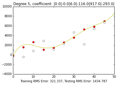

As you can see however, when there is noise in the observations, the higher degree curves would start fitting into the noise. This would cause the training error to be of small value. However, the noise is regenerated again, the curve would be completely inaccurate. As shown in the x axis label, the 8th degree graph has the greatest testing error while the 2nd degree graph has the least testing error as we used a degree 2 polynomial to generate the observations.

This graph shows the direct comparison between the training error(in red) and the testing error(in blue). As you can see, the training error decreases as the degree of the polynomial gets higher and higher. However, the testing error is the greatest at degree eight polynomial and lowest at degree two since the observations were generated from degree two polynomial.
COMPLETE CODE :
What is an observation? An observation is anything that you observe. However, in the real world, it's never possible to measure observations with a 100% accuracy. There will be some fluctuations such as measurement errors or even random changes in the environment that can affect the observations. These random factors that we don't know of and cause fluctuations is called, noise. An observation is a combination of the effect plus the noise.
How would we want to fit the curve into these observations where effect and noise are mixed together? We don't want to fit the curve into the noise since the noise is random and can completely fluctuate. We only want to fit the curve to the effect, but not the noise. However, since we cannot distinguish between them easily, then in this post, we will talk about techniques to handle this.
In this example, let's talk about a polynomial curve fitting. For example, a third degree polynomial is a function in the form of: y = a*x^3 + b*x^2 + c*x + d. As the degree of the polynomial increases, the power of fitting the observations also increases because you would have more parameters to adjust to improve the fitness. For example, in a second degree curve you would have 3 coefficients while, in a third degree curve you would have 4 coefficients. In other words, polynomials with higher degrees contain polynomials with lower degrees by just setting the higher degree coefficients to be 0.
However, would the polynomial get so powerful that it not only fits the real effect, but starts fitting the noise as well? Let's do an experiment to find out. In this experiment, I will do the following:
- Generate the observations based on a 2nd degree polynomial ( this is the underlying relationship of the real effect that we want to discover)
- Generate a random noise using a gaussian distribution which requires the mean (kept at the value 0) and the standard deviation (the noise fluctuates more when you increase the standard deviation)
- Fit curves with different degrees and see which curve fits the best (find the root of the mean of the square of the training error [difference between the observation and the curve prediction]). For example, to fit observations with a degree 2 polynomial, you would adjust the wideness of the parabola, the slope, and the level in order to find the minimal training error.
- Generate some additional observations based on the original formula (This is used to find the testing error)
- Compare the training error and testing error across different degrees of polynomial to determine which degree is best fitting (only fit the effect but not the noise)
Without Noise:
Observations that I generated based on second degree polynomial (3*x^2 + 4*x + 20) with no fluctuation(red).
These graphs have observations without noise in them, meaning that there is no fluctuation. The curve in each graph below is the curve fitted in the given observations. The dots represent the observations that I get without any noise fluctuation:
Since the observations had no noise and fluctuation and was generated using a second degree polynomial, the second degree curve perfectly fits the observations. All degrees higher the second degree curve would also fit the observations perfectly since having more coefficients to adjust would not hurt. The higher degree coefficients could just be set to 0. As you can see in the Degree 5 curve graph the top 3 highest coefficients are 0 since they are not needed in a second degree polynomial. However, since the observations were made from a second degree polynomial, the first degree polynomial did not have enough adjusting power to be able to fit the observations correctly. Therefore there is training error in the degree 1 graph.
With Noise:
These graphs have observations with noise in them, which means that there is fluctuation. The curve in each graph below is the curve fitted in the given observations. In order to fit the observations, the coefficients of the polynomial would be adjusted until the minimal training error is found. In order to minimize the training error, all you have to do is minimize the sum of the square of the differences in each point.
The goal of this experiment is to find a curve that would fit the initial observations(red dots) the best. These observations are made up of the real effect added with some noise. Unfortunately, if the curve fits the red dots well, we do not know whether or not it is just fitting the real effect or also fitting the noise. Because of this, we next add some additional observations such that the curve would not have a chance to fit the white dots. This would allow us to figure out whether or not we are just fitting the real effect or fitting the noise too. In an overfitting situation, the curve would fit the red dots with much less error than the white dots.
The goal of this experiment is to find a curve that would fit the initial observations(red dots) the best. These observations are made up of the real effect added with some noise. Unfortunately, if the curve fits the red dots well, we do not know whether or not it is just fitting the real effect or also fitting the noise. Because of this, we next add some additional observations such that the curve would not have a chance to fit the white dots. This would allow us to figure out whether or not we are just fitting the real effect or fitting the noise too. In an overfitting situation, the curve would fit the red dots with much less error than the white dots.
This graph shows the direct comparison between the training error(in red) and the testing error(in blue). As you can see, the training error decreases as the degree of the polynomial gets higher and higher. However, the testing error is the greatest at degree eight polynomial and lowest at degree two since the observations were generated from degree two polynomial.
COMPLETE CODE :
import random
import pylab
import numpy
import math

def pfunc(a, b, c):
    x = [i*5 for i in range(0, 10)]
    #x = sorted([random.randrange(0, 51) for i in range(0, 10)])
    estx = range(0, 51)
    negylim = -4000
    posylim = 10000
    y = [(a*num**2 + b*num + c)+random.gauss(0, 1000) for num in x]
    y1 = [(a*num**2 + b*num + c)+random.gauss(0, 1000) for num in x]
    pylab.figure('Plot1')
    pylab.ylim(negylim, posylim)
    pylab.plot(x, y, 'ro')

    #Degree 1
    l, m = pylab.polyfit(x, y, 1)
    esty = [(l*num + m) for num in estx]
    estlessy = [(l*num + m) for num in x]
    pylab.figure('Plot2')
    pylab.xlabel('Training RMS Error: '
                +str(round(math.sqrt(numpy.mean([(y[i]-estlessy[i])**2
                for i in range(0, len(estlessy))])), 3))
                + ', Testing RMS Error: '
                +str(round(math.sqrt(numpy.mean([(y1[i]-estlessy[i])**2
                for i in range(0, len(estlessy))])), 3)))
    pylab.title('Degree 1, coefficient: |' + str(round(l)) + '|' + str(round(m)) + '|')
    pylab.ylim(negylim, posylim)
    pylab.plot(x, y, 'ro')
    pylab.plot(x, y1, 'ow')
    pylab.plot(estx, esty, 'g')

    #Degree 2
    l, m, n = pylab.polyfit(x, y, 2)
    esty = [(l*num**2 + m*num + n) for num in estx]
    estlessy = [(l*num**2 + m*num + n) for num in x]
    pylab.figure('Plot3')
    pylab.xlabel('Training RMS Error: '
                +str(round(math.sqrt(numpy.mean([(y[i]-estlessy[i])**2
                for i in range(0, len(estlessy))])), 3))
                + ', Testing RMS Error: '
                +str(round(math.sqrt(numpy.mean([(y1[i]-estlessy[i])**2
                for i in range(0, len(estlessy))])), 3)))
    pylab.title('Degree 2, coefficient: |'
                + str(round(l)) + '|'
                + str(round(m)) + '|'
                + str(round(n)) + '|')
    pylab.ylim(negylim, posylim)
    pylab.plot(x, y, 'ro')
    pylab.plot(x, y1, 'ow')
    pylab.plot(estx, esty)

    #Degree 5
    l, m, n, o, p, q = pylab.polyfit(x, y, 5)
    esty = [(l*num**5 + m*num**4 + n*num**3 + o*num**2 + p*num + q)
            for num in estx]
    estlessy = [(l*num**5 + m*num**4 + n*num**3 + o*num**2 + p*num + q)
                for num in x]
    pylab.figure('Plot4')
    pylab.xlabel('Training RMS Error: '
                +str(round(math.sqrt(numpy.mean([(y[i]-estlessy[i])**2
                for i in range(0, len(estlessy))])), 3))
                + ', Testing RMS Error: '
                +str(round(math.sqrt(numpy.mean([(y1[i]-estlessy[i])**2
                for i in range(0, len(estlessy))])), 3)))
    pylab.title('Degree 5, coefficient: |'
                + str(round(l)) + '|'
                + str(round(m)) + '|'
                + str(round(n)) + '|'
                + str(round(o)) + '|'
                + str(round(p)) + '|'
                + str(round(q)) + '|')
    pylab.ylim(negylim, posylim)
    pylab.plot(x, y, 'ro')
    pylab.plot(x, y1, 'ow')
    pylab.plot(estx, esty, 'y')

    #Degree 8
    l, m, n, o, p, q, r, s, t = pylab.polyfit(x, y, 8)
    esty = [(l*num**8 + m*num**7 + n*num**6 + o*num**5
            + p*num**4 + q*num**3 + r*num**2 + s*num + t)
            for num in estx]
    estlessy = [(l*num**8 + m*num**7 + n*num**6 + o*num**5
                + p*num**4 + q*num**3 + r*num**2 + s*num + t)
                for num in x]
    pylab.figure('Plot5')
    pylab.xlabel('Training RMS Error: '
                +str(round(math.sqrt(numpy.mean([(y[i]-estlessy[i])**2
                for i in range(0, len(estlessy))])), 3))
                + ', Testing RMS Error: '
                + str(round(math.sqrt(numpy.mean([(y1[i]-estlessy[i])**2
                for i in range(0, len(estlessy))])), 3)))
    pylab.title('Degree 8, coefficient: |'
                + str(round(l)) + '|'
                + str(round(m)) + '|'
                + str(round(n)) + '|'
                + str(round(o)) + '|'
                + str(round(p)) + '|'
                + str(round(q)) + '|'
                + str(round(r)) + '|'
                + str(round(s)) + '|'
                + str(round(t)) + '|')
    pylab.ylim(negylim, posylim)
    pylab.plot(x, y, 'ro')
    pylab.plot(x, y1, 'ow')
    pylab.plot(estx, esty, 'm')


pfunc(3, 4, 20)
No comments:
Post a Comment